March 2, 2023
Studying basic Latin using Ascham’s method
When I first searched for a Latin textbook in 2019 I assumed that a text published in 1886, “The Beginner’s Latin Book” by Collar and Daniell, would be an excellent choice since schools at the time took the classics seriously and produced students capable of enjoying Caesar & Livy within the first few years of instruction. However, Collar and Daniell warn in the preface to their work “those who seek in a first Latin book a complete presentation of the facts and principles of the Latin language will not be satisfied with this volume” and the authors only “hope” that the transition to Nepos or Caesar “will not prove too difficult.” Collar and Daniell include these warnings because it was precisely in the 1880s that the number of American high schools was increasing by 400 annually and the number of subjects taught in high school was multiplying to include sciences and modern history. Collar and Daniell, catering to the new American high school, reduced their text’s demands on the students’ time and energy and on the teachers’ ability and knowledge of Latin, allowing students to study more subjects shallowly and allowing teachers to be rapidly trained to teach first-year Latin by staying one chapter ahead of their class. Because of its design, Collar and Daniell’s revision to their 1886 text called “First Year Latin” was used in more schools in America from 1890 until 1910 than all other competing Latin texts combined. I believe the text is still a good choice, despite being the product of compromise, for those with limited time or motivation.
Unlike Collar & Daniell’s approach of introducing piecemeal various grammatical forms (nominative of 1st declension nouns and the 3rd person of 1st conjugation verbs in Ch. 1, the accusative of 1st declension nouns in Ch. 2, etc.), traditional methods of teaching Latin in use for over 1000 years involved students memorizing over the course of several weeks a full Latin grammar organized like the Ars Minor of Donatus (written in the 4th Century) and the Institutiones Grammaticae of Priscian (6th Century). These grammars resemble Lily’s Latin Grammar, the main text used in America and British schools during the 16th through 19th centuries–effectively an English rendering of Donatus and Priscian–in that they first definite parts of speech, then treat nouns exhaustively, then adjectives, then verbs, etc. Consider the first few sentences of Donatus in Latin and in English translation:
Partes orationis quot sunt? Octo. Quae? Nomen pronomen verbum adverbium participium coniunctio praepositio interiectio.
Nomen quid est? Pars orationis cum casu corpus aut rem pro- prie communiterve significans. Nomini quot accidunt? Sex.
— English translation of the above: —
How many parts of speech are there? Eight. What? Noun, pronoun, verb, adverb, participle, conjunction, preposition, interjection.
What is a noun? A part of speech which signifies with the case a person or a thing specifically or generally. How many attributes has a noun? Six.
This style of exhaustive grammar is dry but makes the aforementioned texts suitable as references. Once such a grammar was memorized by a class, a teacher would present his class with a text in Latin, produce a translation, parse words and explain syntax. Later, students would be tested by being given the translation and asked to reproduce the original Latin, a process which encouraged many students to simply memorize the passages instead of developing a skill of “construing” Latin. However, memorization served the students well in becoming competent Latinists.
A better method of teaching Latin, according to Roger Ascham in his “The Scholemaster”, avoids memorizing a complete grammar and has a teacher read sophisticated Latin to his class right away while explaining every grammatical point to his students and showing where the rule appears in their thorough grammars. As Ascham says “This is a liuely and perfite waie of teaching of Rewles: where the common waie, vsed in common Scholes, to read the Grammer alone by it selfe, is tedious for the Master, hard for the Scholer, colde and vncomfortable for them bothe.” As a first text, Ascham recommended a schoolmaster use a compilation of Cicero’s letters created by Johannes Sturm for beginning students in which letters are presented in a graded format starting with very simple and short letters and getting longer and more difficult further into the collection. It’d be easier to go through these letters with the help of an experienced Latinist, of course, but I’m going to attempt reading, translating and annotating with grammatical references Sturm’s collection of letters. The standard grammar I’ll use will either be Gildersleeve’s or a later edition of Lily’s Grammar.
September 11, 2020
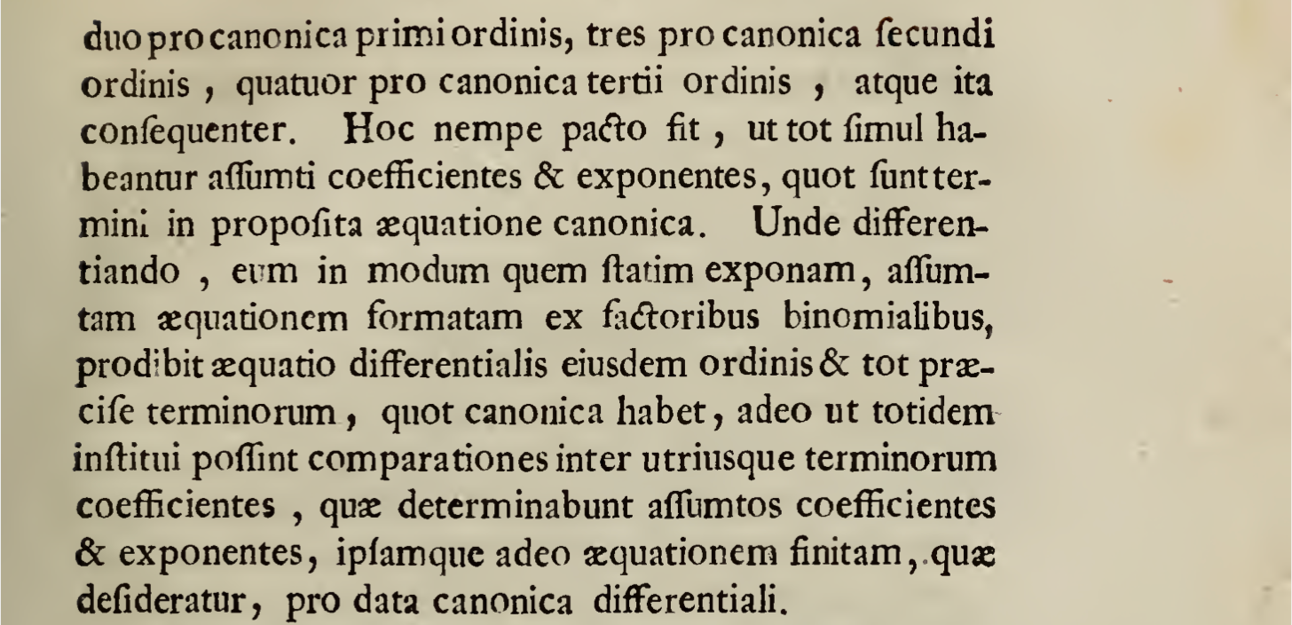
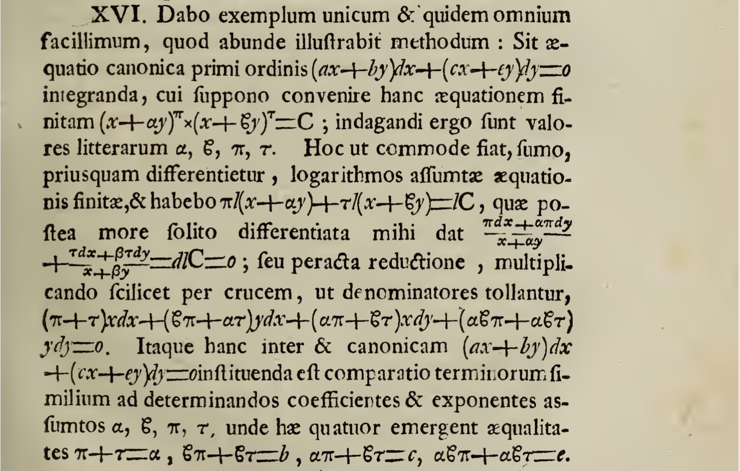
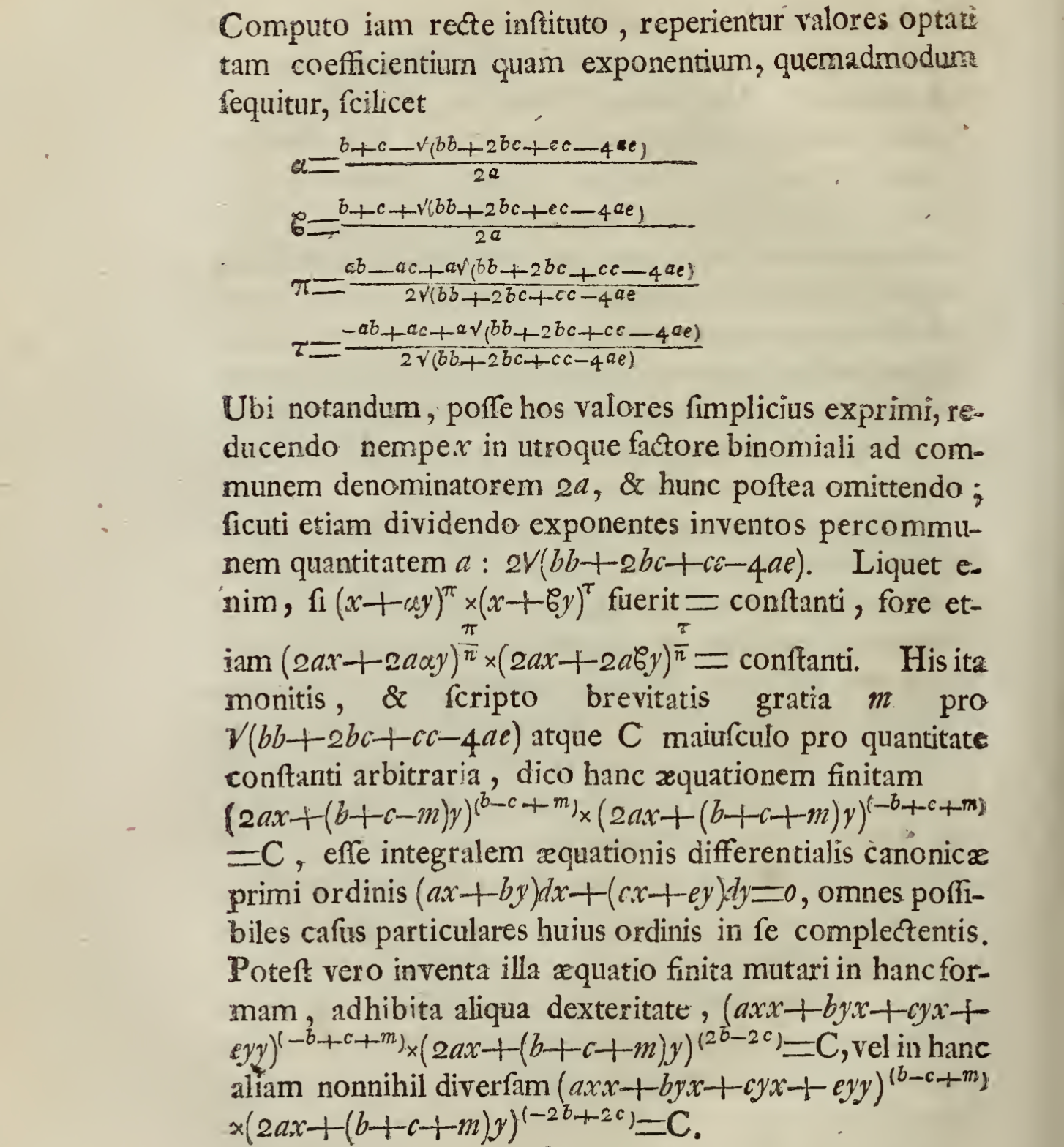
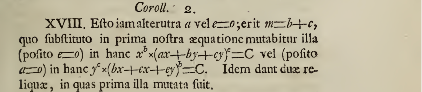
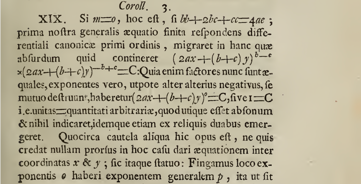
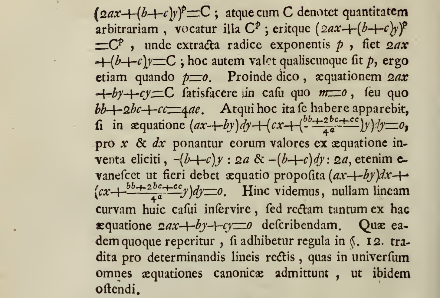
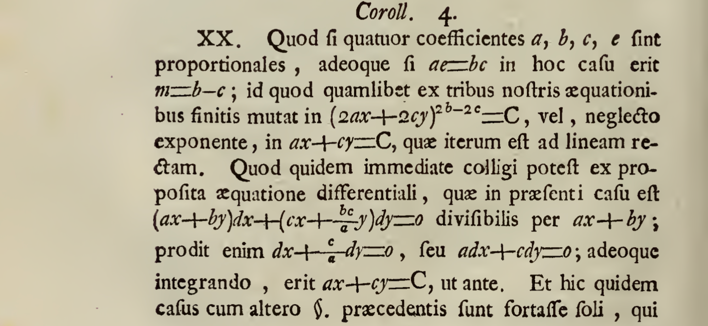
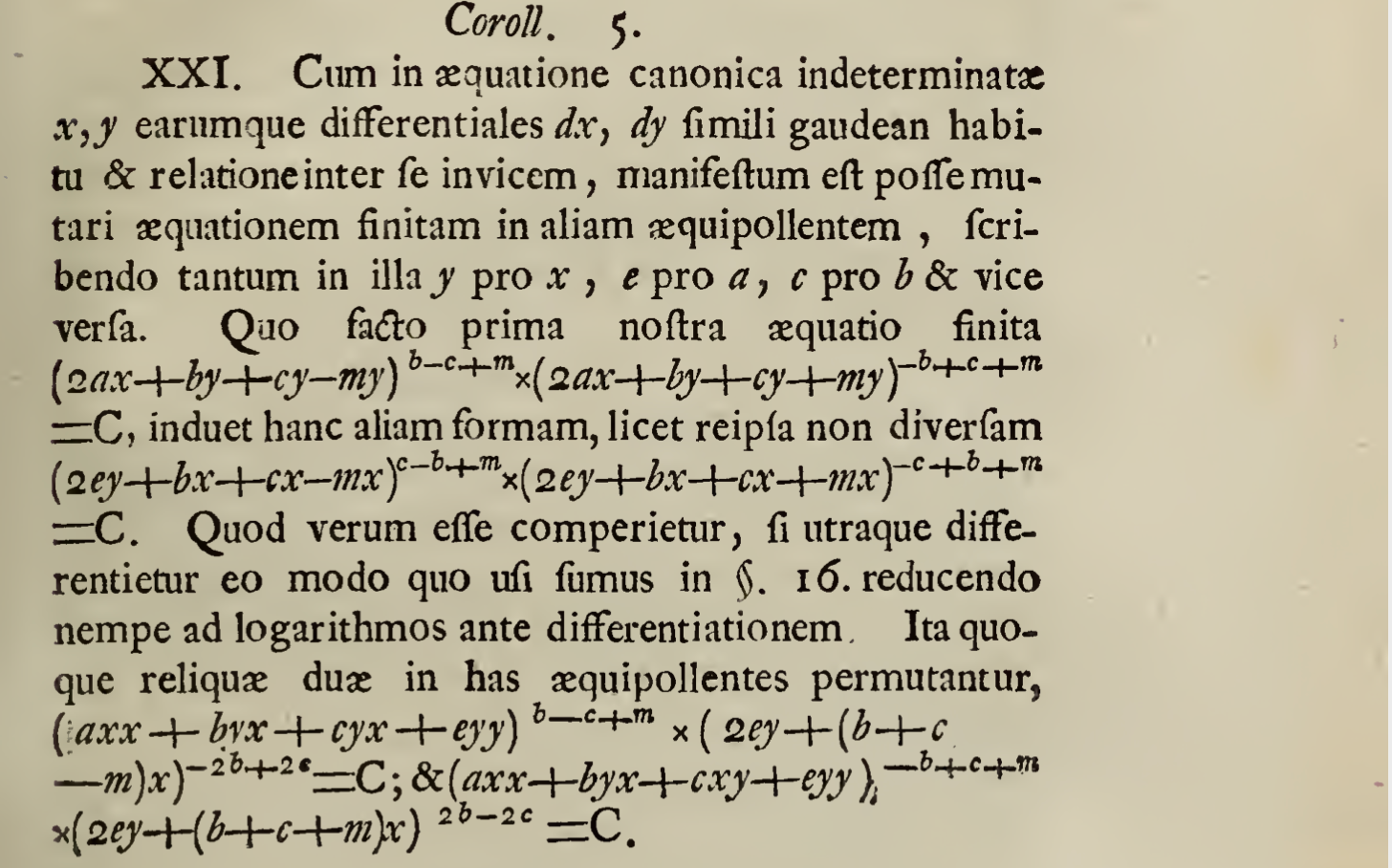
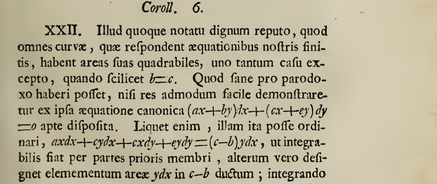
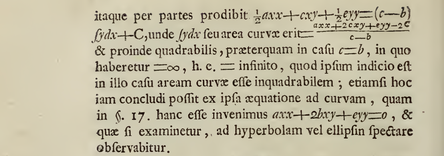
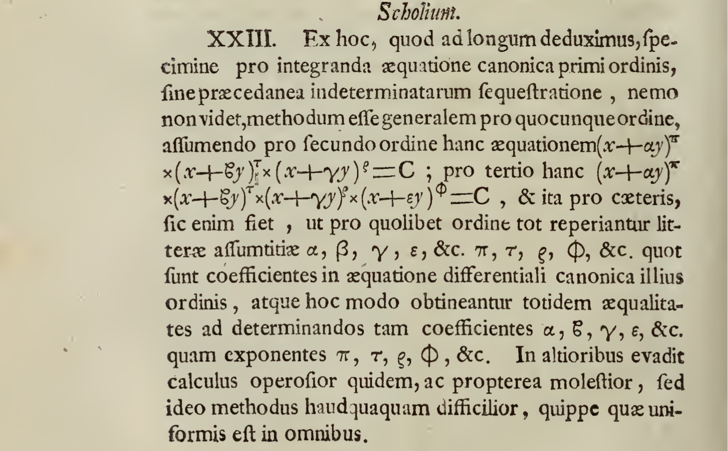
De integraionibus aequationum differentialium
On the integration of differential equations
Where an example of a method of integrating without earlier separation of variables is recounted.
Author Johann Beroulli, June 1726
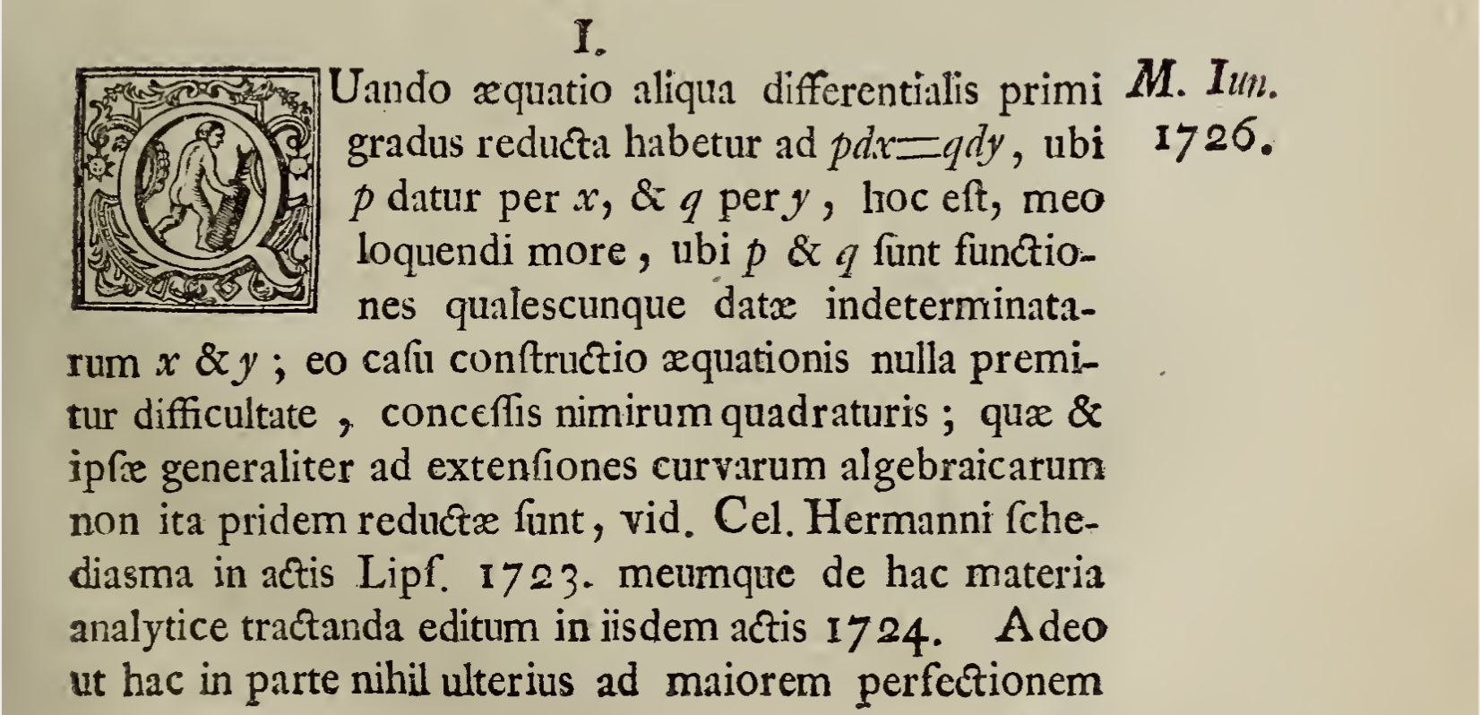
1.
When any first degree differential equation has been reduced to pdx=qdy, ubi p datur per x, & q per y, that is, in my manner of speaking, ubi p & q are any functions given by the indeterminates x & y; in this case, the construction of the equation poses no difficulty, (including of course second order equations); which can be generalized to extensions of algebraic curves which were not first reduced, see Cel. Hermanni’s article in Acta Eruditorum of Liepzig, 1723. I also treated this analytic material in the same journal’s 1724 publication.
To go in this way in no
utpote === namely, as , since
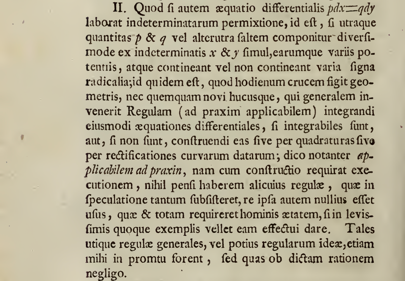
2.
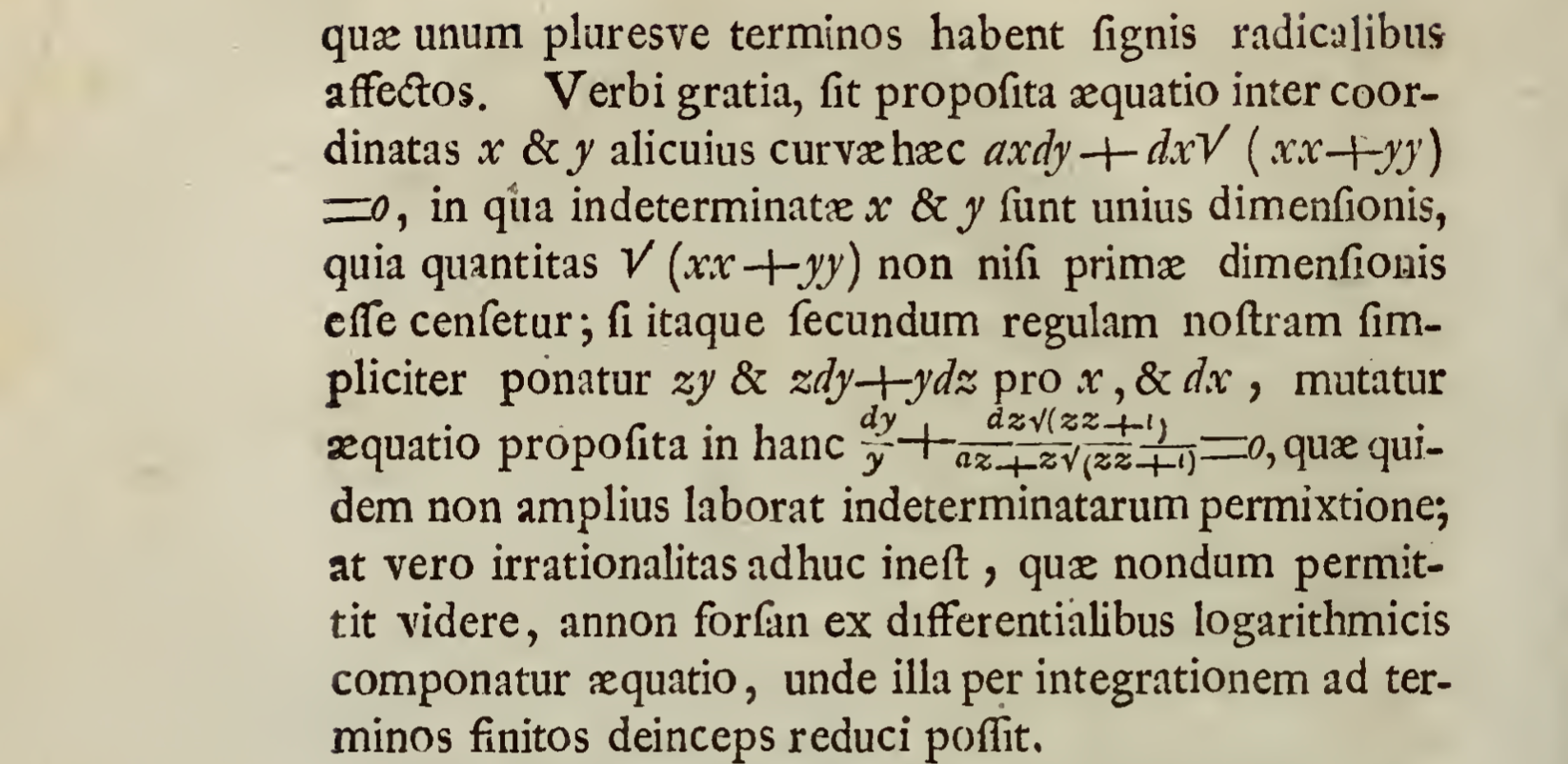
Moreover, if because the differential equation pdx=qdy is produced with mixed indeterminates, that is, if both quantities p & q or one of the two at least are diversely composed of the indeterminates x & y simultaneously, and of these different powers, or containing or not containing different radical signs; it indeed is
hūcusque (not comparable) === up to this point, until now
3.
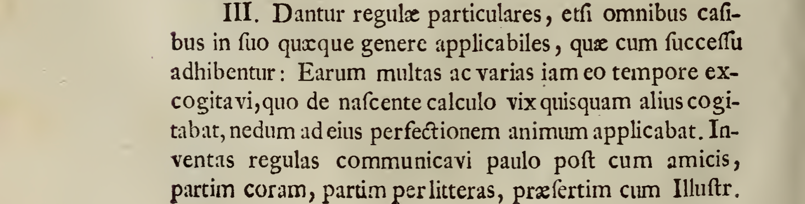
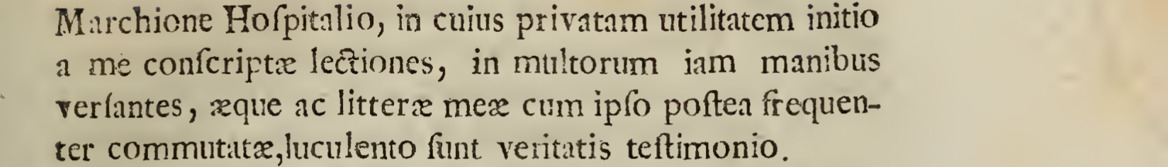
Given particular rules, even if all cases in which are generally applicable, which are applied.
Marquis de l’Hôpital,
4.
5.
6.
7.
8.
9.
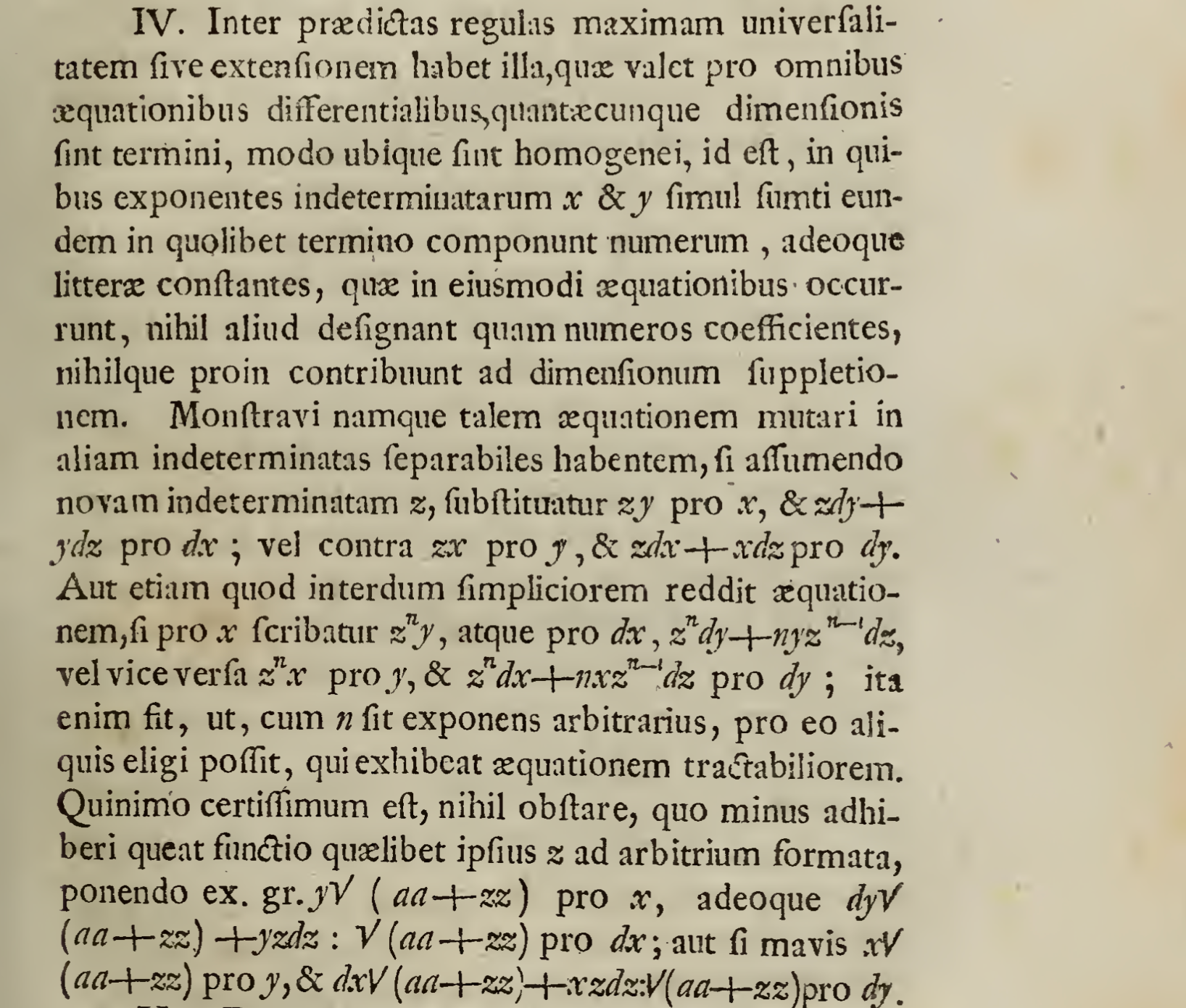
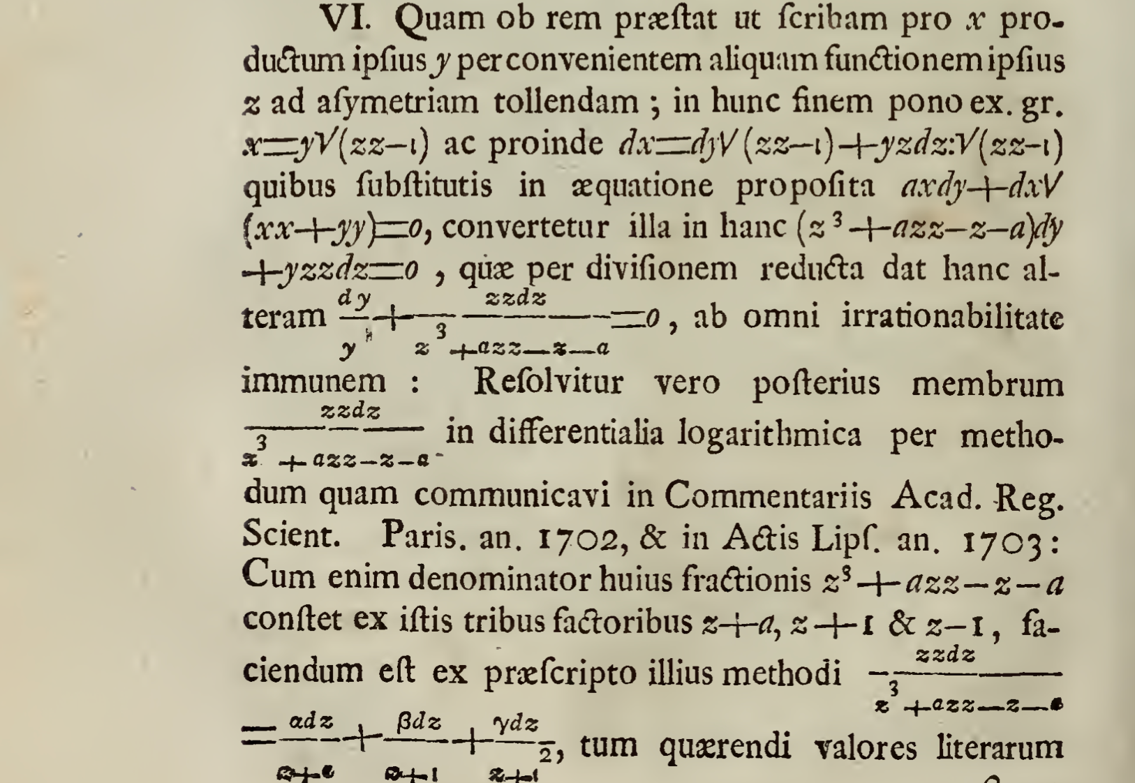
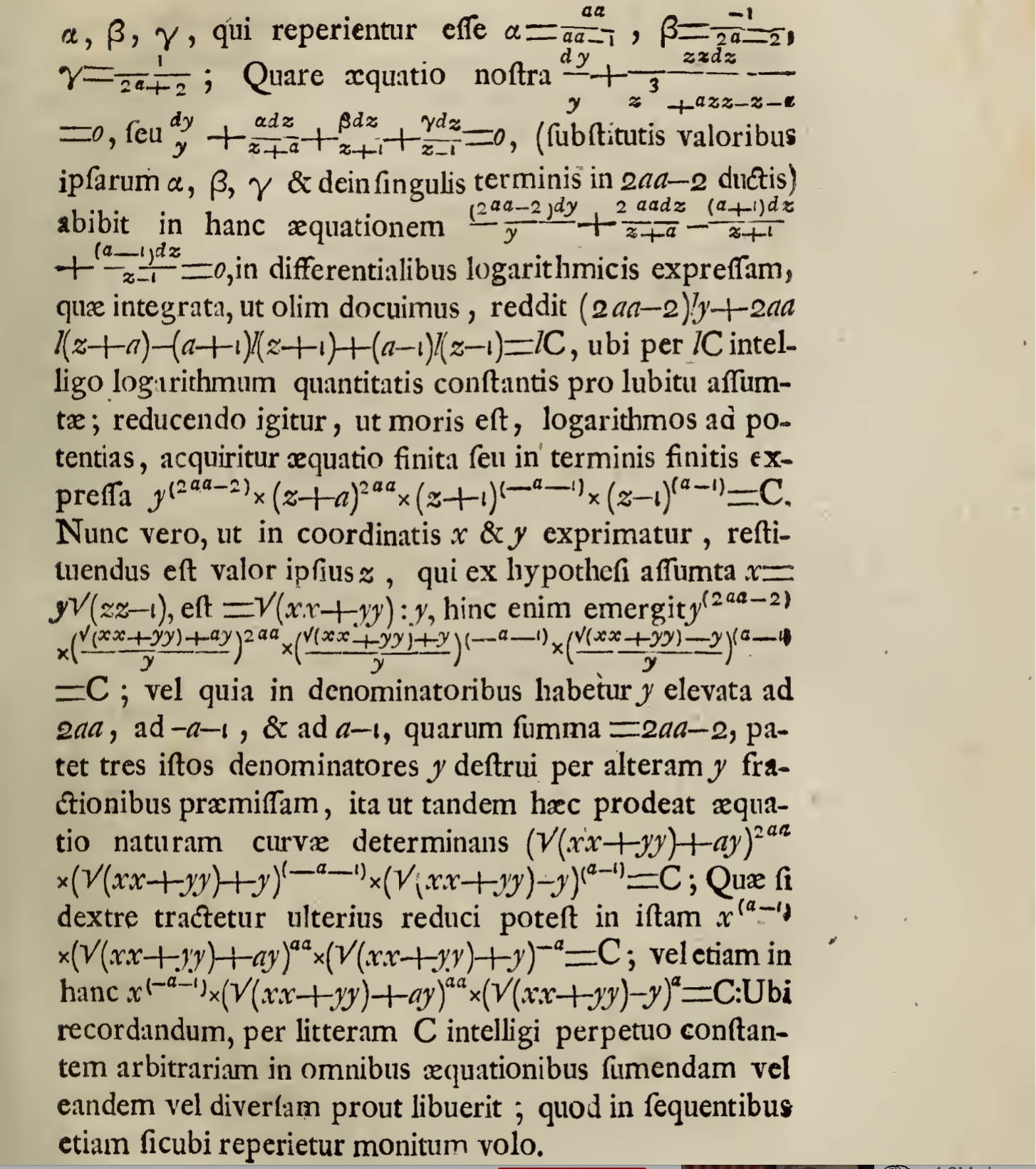
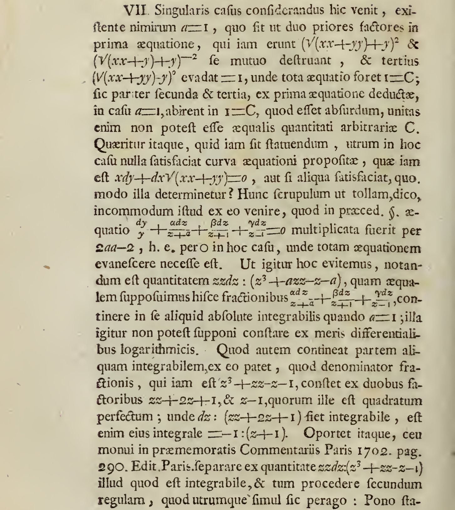
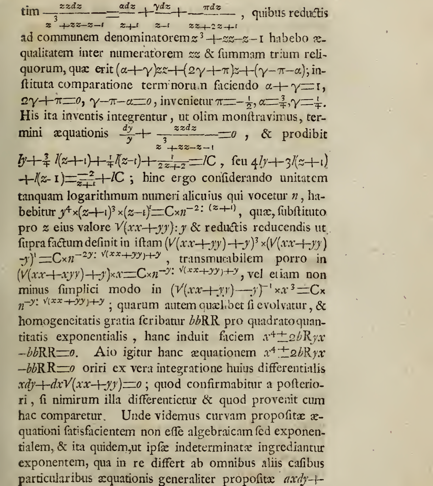
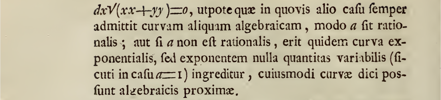
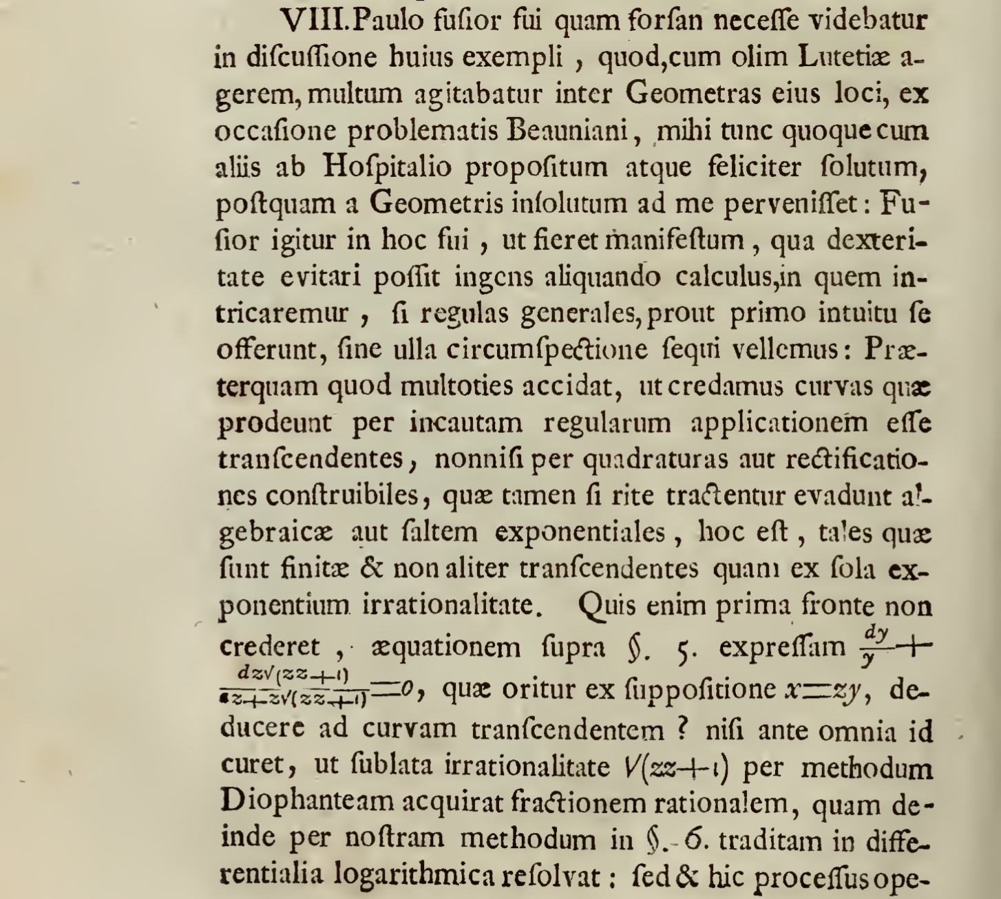
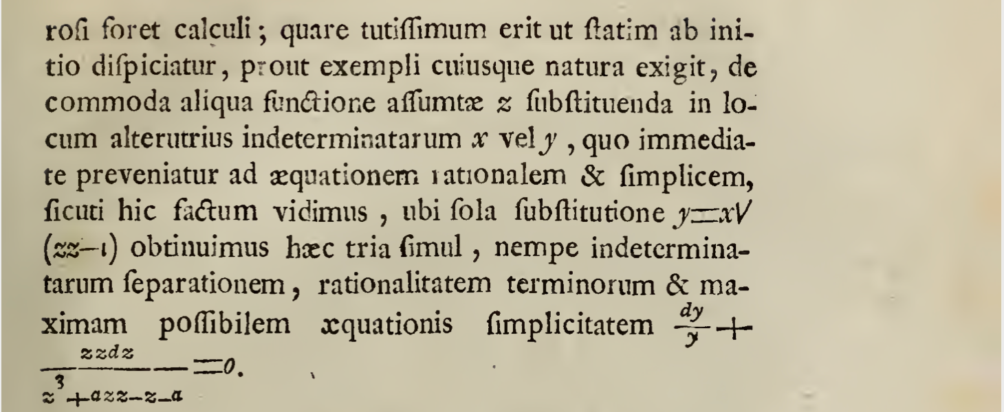
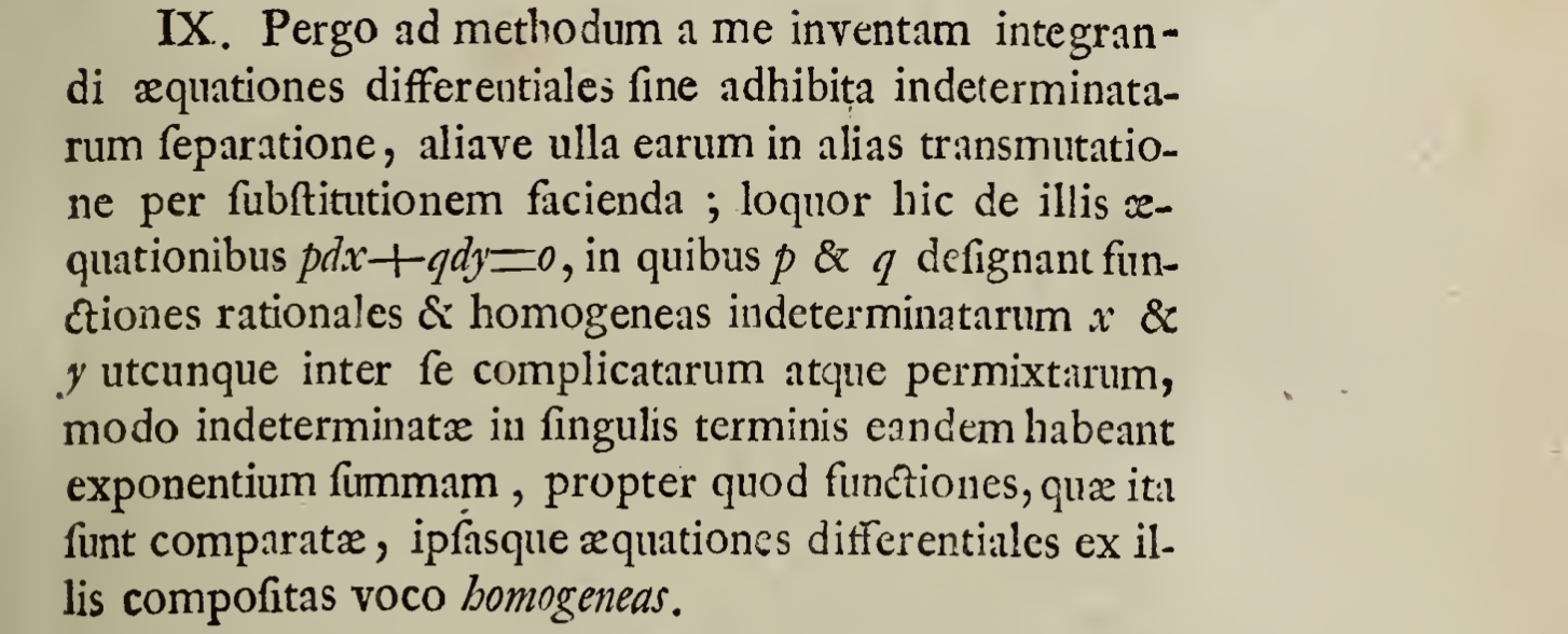
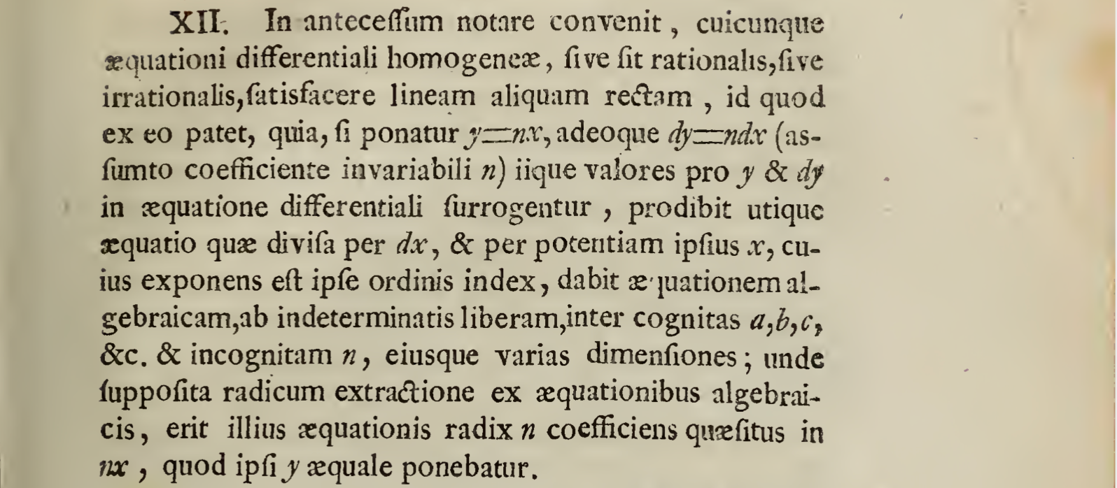
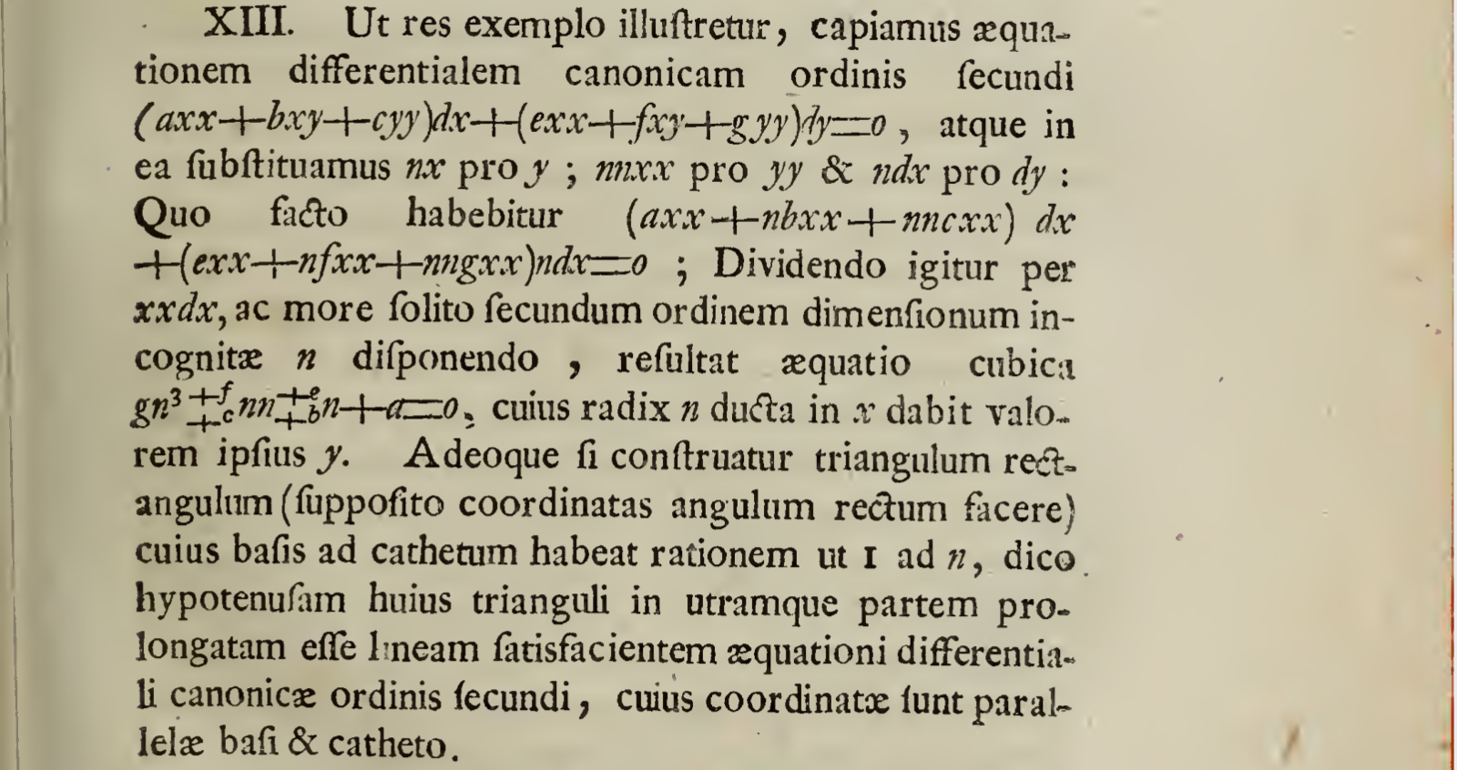
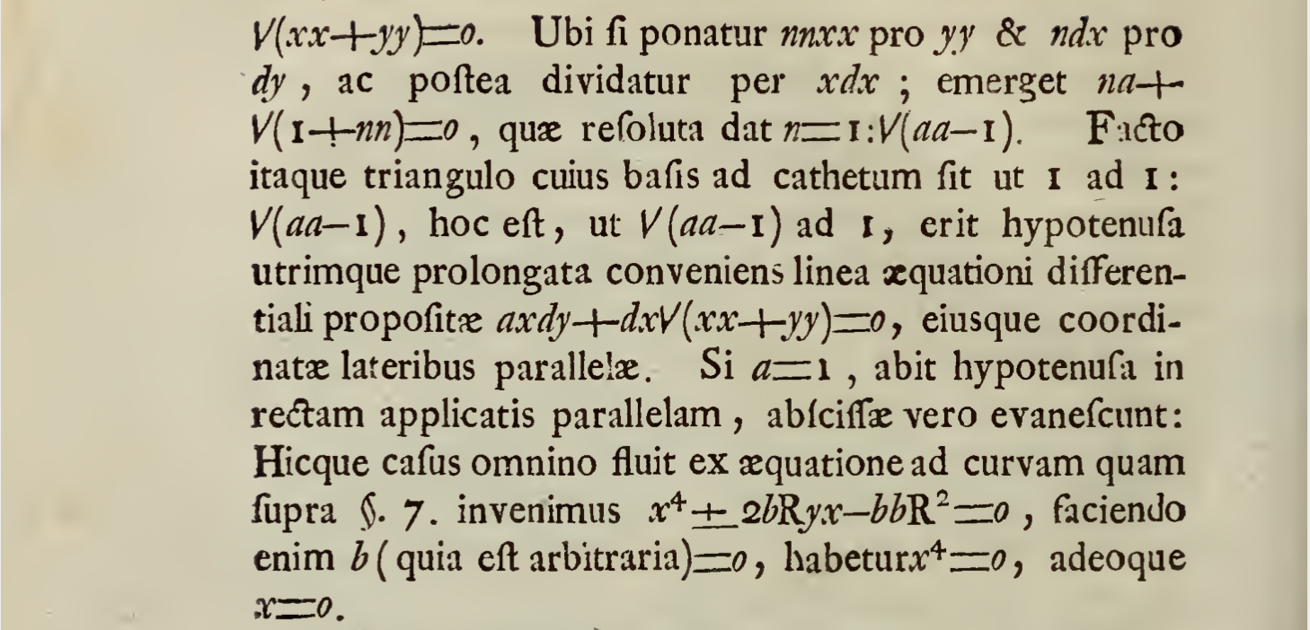
I proceed to the method invented by myself to the integratino of differential equations without the use of separation of indeterminates, any of them in another transmutation made by substitution; I say here of these equations pdx+qdy=0, in which p & q indicate rational, homogeneous functions of the indeterminates x & y however between them complicated and mingled, only the indeterminates in every end having the same exponent, because these functions, of which are so prepared, these very differential equations which are composed of these I call homogeneous.
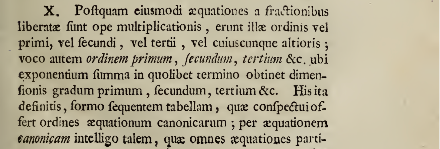
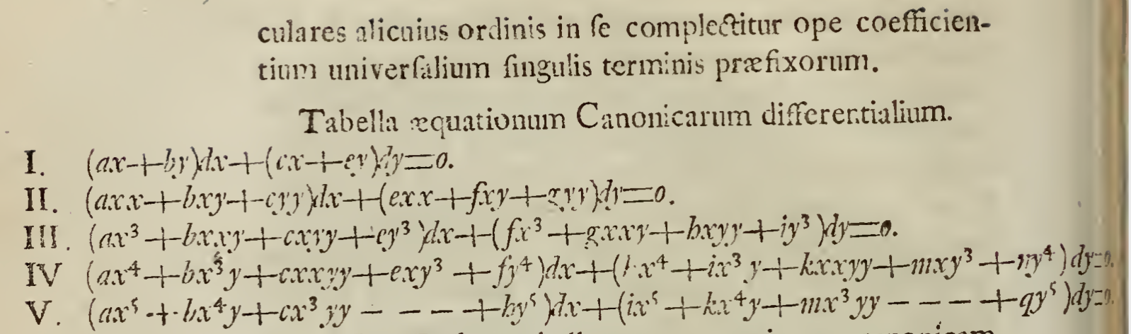
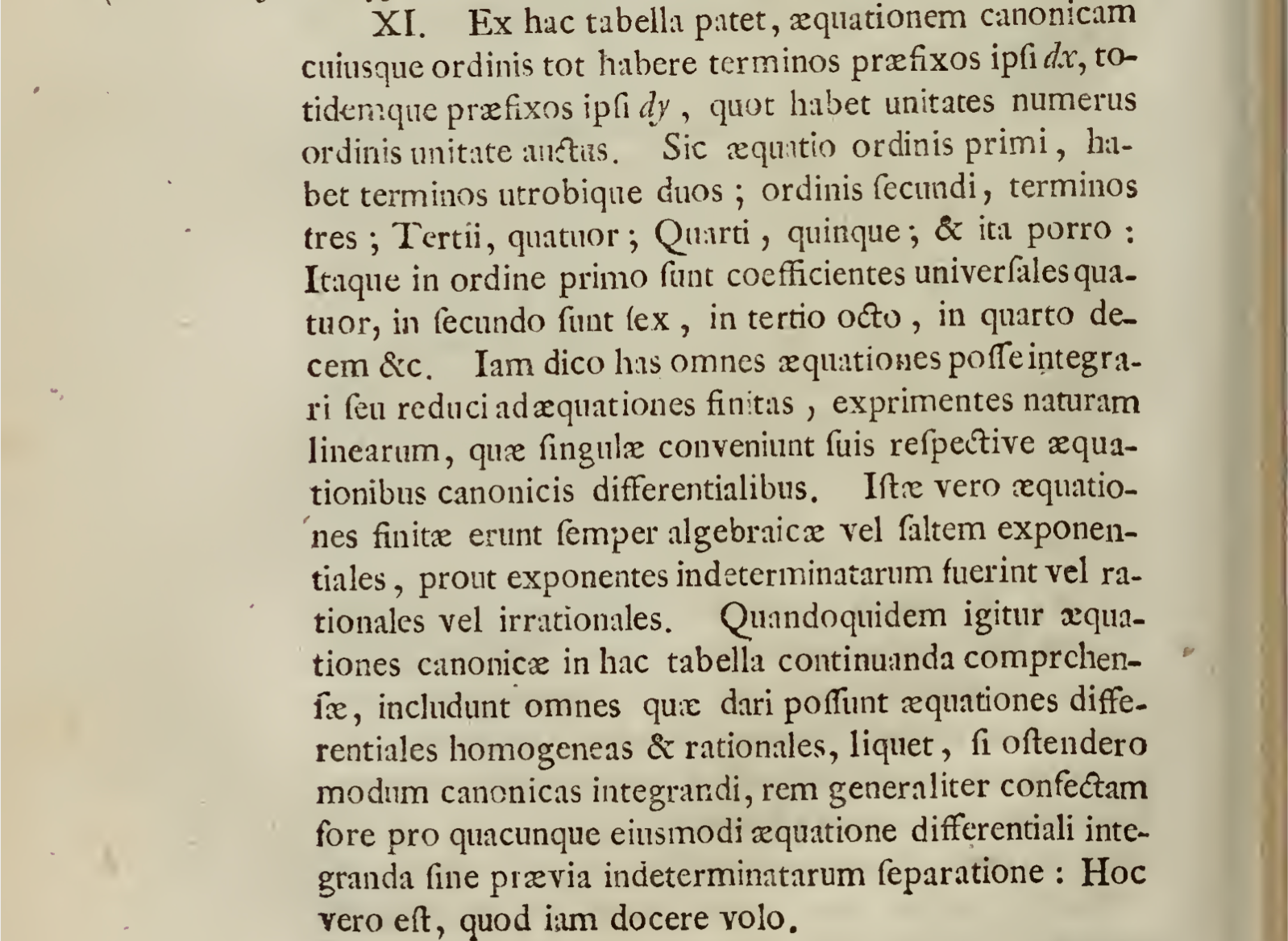
10.


September 17, 2018
Arithmetic on a very small elliptic curve
This document gives a detailed illustration of discrete elliptic curve mathematics. After reading this document, one should be able to carry out calculations on elliptic curves by hand. The document is broken down as follows:
- Introduction to a small curve and a discussion of “points at infinity”
- Examples of adding points on elliptic curves over finite fields
- Demonstration of how to use sage to do basic computations on elliptic curves
For those lacking background on elliptic curves, Andrea Corbellini’s gentle introduction to elliptic curve cryptography should be read first.
Elliptic curves
In a cryptographic setting–we’ll avoid abstract mathematics for now–an elliptic curve is any polynomial equation of the form
y2=x3+Ax+B
Where A,B∈F and F is some field.
Bitcoin’s curve
Satoshi chose a curve called secp256k1 for Bitcoin’s elliptic curve public key cryptography. The curve has the form
y2=x3+7
where all coefficients and arithmetic operations are over the finite field Fp,p=2256−4294968273 (i.e. the field whose elements are the integers modulo p).
Same curve, different field
The field used in secp256k1 is too big for manual calculations so we’ll consider a curve over the smaller field of integers modulo 13. Any solution (x,y) to the polynomial equation y2=x3+7 (mod 13) are points on the elliptic curve defined by this equation. This small elliptic curve has order 7 and these are the 7 points on the curve:
{∞,(7,5),(7,8),(8,5),(8,8),(11,5),(11,8)}
The points of the curve form a cyclic group which implies that all points, excluding ∞, the identity, are generators of the curve, i.e. if any of these points are repeatedly added to themselves, all points of the curve will eventually be generated. The points of the standard curve secp256k1 are also generators, again excluding ∞.
Point at infinity
In homogeneous coordinates for projective space, the equation of our small elliptic curve becomes
y2z=x3+7z3
In homogeneous coordinates, points, including points at infinity, can be represented using only finite coordinates. Absolute magnitudes do not matter; only ratios of magnitudes matter. Without loss of generality, we can normalize the last nonzero entry of coordintes (x:y:z) to 1. By setting z=1 in the equation above, we get our original equation of the curve. Due to normalization, the only other option is to consider the case where z=0.
y2⋅0=x3+7⋅0
For this expression to hold, y can be any value while x must equal 0. Normally, we consider only a single “point at infinity” with coordinates (0:1:0). Why these coordinates in particular? As we explained above, if z is nonzero, it can be normalized to 1, but when we take z=0, we must have x=0 while y can be an arbitrary integer; again, we choose to normalize y to 1. If we consider z to be in the denominator of a ratio, than the convention of division by zero producing infinity, x/0=∞, gives some intuition about why the point is considered to be “at infinity”. We work in affine coordinates for the rest of this document so we’re forced to represent the point at infinity as ∞.
Point addition on an elliptic curve over a finite field
Let P=(7,5) and Q=(8,8).
Root trick
We use the following observation in the two calculations below. Notice that when a cubic polynomial is factored each of the roots appear in the three factors. If the polynomial is expanded.
y2=(x−a)(x−b)(x−c)=(x2−(a+b)x+ab)(x−c)=x3−(a+b)x2+abx+cx2+c(a+b)x−abc=x3−(a+b+c)x2+(ab+ac+bc)x−abc
So the coefficient of x2 is the sum of the three roots of the elliptic curve.
Adding two distinct points
We solve for R=P+Q=(7,5)+(8,8).
First, we find the slope of the line joining the two points.
m=8−78−5=3
Then we find the equation of the line by substituting the coordinates of P into the equation of a line with the slope calculated above.
y=3(x−7)+5=3x−16≡3x−3≡3x+10
Now we substitute the equation of the line into the formula for the curve.
y2=(3x+10)2=9x2+60x+100=x3+7 ⟹0=x3−9x2−60x−93
Using the root trick, 9=7+8+x≡15+x≡2+x⟹x=7 (7 and 8 being the x-coordinates of P and Q). Then we substitute this value of x into our equation of the line.
y=3x+10=31≡5
Finally we reflect this value for y to find −y=−5≡8. Therefore P+Q=(7,5)+(8,8)=(7,8).
Adding a point to itself
To find S=P+P we first calculate the tangent line to P=(7,5) using implicit differentiation on the equation of the curve y2=x3+7.
2yy′=3x2⟹y′=2y3x2=2⋅53⋅72=10147=104=4(10−1)=4⋅4=16≡3
Then we find the equation of the line by substituting the coordinates of P into the equation of a line with the slope (y′=m) calculated above.
y=3(x−7)+5=3x−16≡3x−3≡3x+10
(Note: the tangent line we found has the exact same slope as the line we found above!)
Now we substitute the equation of the line into the formula for the curve.
y2=(3x+10)2=9x2+60x+100=x3+7 ⟹0=x3−9x2−60x−93
Using the root trick, 9=7+7+x≡14+x≡1+x⟹x=8. Then we substitute this value of x into our equation of the line.
y=3⋅8+10=24≡8
Finally we reflect this value for y to find −y=−8≡5. Therefore P+P=(7,5)+(7,5)=(8,5).
Verification of results in Sage
Using sage REPL to verify our results above.
sage: F = FiniteField(13); F
>>> Finite Field of size 13
sage: E = EllipticCurve(F, [ 0, 7]); E
>>> Elliptic Curve defined by y^2 = x^3 + 7 over Finite Field of size 13
sage: E.points()
>>> [(0 : 1 : 0), (7 : 5 : 1), (7 : 8 : 1), (8 : 5 : 1), (8 : 8 : 1), (11 : 5 : 1), (11 : 8 : 1)]
sage: P = E.point((7,5)); P
>>> (7 : 5 : 1)
sage: P.order()
>>> 7
sage: Q = E.point((8,8)); Q
>>> (8 : 8 : 1)
sage: Q.order()
>>> 7
sage: P + Q
>>> (7 : 8 : 1)
sage: P + P
>>> (8 : 5 : 1)
May 16, 2018
Keccak implementation in Haskell
A Haskell programmer typically relies on cryptonite for hash implementations. cryptonite is exhaustive and efficient; most of its cryptographic functions are implemented in C and invoked using Haskell’s FFI. This week, I finished an implementation of the Keccak hash (SHA3) in pure Haskell which I needed for a project of mine compiled with ghcjs (ghcjs cannot compile Haskell which uses the C FFI.)
While researching Keccak, I learned that much more than hashes could be implemented using its underlying “sponge” construction. The Keccak team writes in their paper Cryptographic Sponge Functions,
In the context of cryptography, sponge functions provide a particular way to generalize hash functions to more general functions whose output length is arbitrary. A sponge function instantiates the sponge construction, which is a simple iterated construction building a variable-length input variable-length output function based on a fixed length permutation (or transformation). With this interface, a sponge function can also be used as a stream cipher, hence covering a wide range of functionality with hash functions and stream ciphers as particular points.
The goals for this keccak library are to implement the hashes, MACs, extendible-output functions, & stream ciphers described by the Keccak team in full generality and in pure, readable Haskell. Currently, the library mainly implements the four standard hashes (224-, 256-, 384-, & 512-bit) for both SHA3 and Keccak (which differ only in padding rules). The implementations are unoptimized so, for context, cryptonite’s C-based implementation of Keccack256 is 21 times faster than my naive, unoptimized Haskell.
benchmarked keccak
time                 768.3 μs   (758.7 μs .. 775.7 μs)
                     0.998 R²   (0.995 R² .. 0.999 R²)
mean                 774.2 μs   (767.5 μs .. 784.0 μs)
std dev              29.27 μs   (23.12 μs .. 36.87 μs)
variance introduced by outliers: 19% (moderately inflated)

benchmarked cryptonite-keccak
time                 36.92 μs   (35.95 μs .. 38.03 μs)
                     0.996 R²   (0.995 R² .. 0.998 R²)
mean                 36.27 μs   (35.99 μs .. 36.66 μs)
std dev              1.147 μs   (918.3 ns .. 1.471 μs)
variance introduced by outliers: 14% (moderately inflated)
Eventually, I hope the library will have very few dependencies (only base, vector & bytestring, currently) and excellent performance.
Example usage
In the example usage below, I encode ByteStrings in base16 so that they can be read as standard hex strings.
ghci> import Data.ByteString.Base16 as BS16

ghci> :t keccak256
keccak256 :: BS.ByteString -> BS.ByteString

ghci> BS16.encode $ keccak256 "testing"
"5f16f4c7f149ac4f9510d9cf8cf384038ad348b3bcdc01915f95de12df9d1b02"

ghci> BS16.encode $ keccak256 ""
"c5d2460186f7233c927e7db2dcc703c0e500b653ca82273b7bfad8045d85a470"
Keccak Background
According to Jean-Philippe Aumasson, the recent winner of NIST’s SHA3 competition, Keccak, is named after the Balinese dance Kecak. Wikipedia offers the following the description of the performance:
Also known as the Ramayana Monkey Chant, the piece, performed by a circle of at least 150 performers wearing checked cloth around their waists, percussively chanting “chak” and moving their hands and arms, depicts a battle from the Ramayana. The monkey-like Vanara led by Hanuman helped Prince Rama fight the evil King Ravana. Kecak has roots in sanghyang, a trance-inducing exorcism dance.[2]
A helpful answer on crytpo.stackoverflow points out that this continues djb’s tradition of naming cryptographic functions after dances. djb chose only Latin dances for his Salsa, Rumba, and ChaCha algorithms.
The Sponge Construction
I quote the paper Cryptographic Sponge Functions again:
The sponge construction is a simple iterated construction for building a function F with variable-length input and arbitrary output length based on a fixed-length transformation or permutation f operating on a fixed number b of bits. Here b is called the width. The sponge construction operates on a state of b = r + c bits. The value r is called the bitrate and the value c the capacity.
In the case of the standard Keccak and SHA3 hashes, the sponge state always has width b = 1600, and it is operated on by the permutation KeccakF[1600] which maps the 1600-bit states to 1600-bit states. What mainly distinguishes SHA3-224 from SHA3-256, SHA3-384, and SHA3-512 is not the output length (which can be made arbitrarily long using the sponge construction), but rather the bitrate r of the hash and its capacity c. Because b = 1600 = r + c, the capacity of the hash must decrease as the bitrate increases and vice versa; a higher bitrate promises better performance while a higher capacity provides better security guarantees. The general operation of the sponge is described by the Keccak team very succinctly:
First, all the bits of the state are initialized to zero. The input message is padded and cut into blocks of r bits. The sponge construction then proceeds in two phases: the absorbing phase followed by the squeezing phase.
- In the absorbing phase, the r-bit input message blocks are XORed into the first r bits of the state, interleaved with applications of the function f. When all message blocks are processed, the sponge construction switches to the squeezing phase.
- In the squeezing phase, the first r bits of the state are returned as output blocks, interleaved with applications of the function f. The number of output blocks is chosen at will by the user. The last c bits of the state are never directly affected by the input blocks and are never output during the squeezing phase.
The keccak library implements the constituant parts of the KeccakF[1600] function using very simple Haskell; hopefully, those new to Keccak can read it more easily than existing C or Python implementations to get a feel for this very simple permutation at the heart of SHA3.
Demonstrating the poor security of low-capacity sponge-based hashes
A second-preimage attack in this example shows that for a keccak hash with capacity c = 32 and bitrate r = 1568, two preimages can be found which both hash to 0xdec1. The attack requires checking only 5544 inputs.
First preimage:
In the context of cryptography, sponge functions provide a particular way to generalize hash functions to more general functions whose output length is arbitrary. A sponge func- tion instantiates the sponge construction, which is a simple iterated construction building a variable-length input variable-length output function based on a fixed length permutation (or transformation). With this interface, a sponge function can also be used as a stream ci- pher, hence covering a wide range of functionality with hash functions and stream ciphers as particular points. From a theoretical point of view, sponge functions model in a very simple way the finite memory any concrete construction has access to. A random sponge function is as strong as a random oracle, except for the effects induced by the finite memory. This model can thus be used as an alternative to the random oracle model for expressing security claims. From a more practical point of view, the sponge construction and its sister construction, called the duplex construction, can be used to implement a large spectrum of the symmetric cryptography functionality. This includes hashing, reseedable pseudo random bit sequence generation, key derivation, encryption, message authentication code (MAC) computation and authenticated encryption. This provides users with a lot of functionality from a single fixed permutation, hence making the implementation easier. The designers of cryptographic primitives may also find it advantageous to develop a strong permutation without worrying about other components such as the key schedule of a block cipher.
Second preimage:
kI!the context of cryptography, sponge functions provide a particular way to generalize hash functions to more general functions whose output length is arbitrary. A sponge func- tion instantiates the sponge construction, which is a simple iterated construction building a variable-length input variable-length output function based on a fixed length permutation (or transformation). With this interface, a sponge function can also be used as a stream ci- pher, hence covering a wide range of functionality with hash functions and stream ciphers as particular points. From a theoretical point of view, sponge functions model in a very simple way the finite memory any concrete construction has access to. A random sponge function is as strong as a random oracle, except for the effects induced by the finite memory. This model can thus be used as an alternative to the random oracle model for expressing security claims. From a more practical point of view, the sponge construction and its sister construction, called the duplex construction, can be used to implement a large spectrum of the symmetric cryptography functionality. This includes hashing, reseedable pseudo random bit sequence generation, key derivation, encryption, message authentication code (MAC) computation and authenticated encryption. This provides users with a lot of functionality from a single fixed permutation, hence making the implementation easier. The designers of cryptographic primitives may also find it advantageous to develop a strong permutation without worrying about other components such as the key schedule of a block cipher.
Testing
NIST uses the Secure Hash Algorithm Validation System (SHAVS) to validate the correctness of hash implementations. For all four variants of SHA3 and Keccak, the keccak library’s implementations successfully pass the standard KATs (Known Answer Tests).
April 5, 2016
Eliminating explicit parentheses with a handy combinator
This is a literate Haskell post about a trick I picked up in Raymond Smullyan’s “To Mock a Mockingbird”, a fantastic introduction to combinator logic.
Let’s start with a simple demonstration. Consider the expression for u:
u = (:) 'g' (show 13)
u evaluates to:
ghci> u
"g13"
Using only function application and the non-infix compose function, I’d like to write a point-free function solution such that the u' defined below evaluates to the same value as u.
u' = solution (:) 'g' show 13
The body of u' differs from u in that show 13 is no longer surrounded by parentheses and a function solution is being applied to the cons function.
We solve for u' by working backwards while thinking about the implicit parentheses we usually leave out when working with curried functions. We also use a synonym for (.) so we’re not overwhelmed by parentheses.
b = (.)
The B combinator in combinator logic is defined B x y z = x (y z) and serves the same purpose as the compose operator in Haskell. The mechanical transformation we use in this post can eliminate parentheses not implied by left-associative function application by using the definition of B to carry out the transformation x (y z) => B x y z. By prefixing an expression with B, we’re able to eliminate a pair of parentheses! We solve
u2 = ((:) 'g') (show 13)
u3 = ((b ((:) 'g')) show) 13
u4 = ((((b b) (:)) 'g') show) 13
u5 = b b (:) 'g' show 13
Therefore,
solution = b b
We can verify that this definition of solution makes u and u' evaluate to identical values.
ghci> u'
"g13"
More generally, this mechanical procedure can transform an arbitrary, properly typed expression with explicit parentheses, e.g.
exp = z (a b) (c (d e) f) (g h i)
to a form entirely devoid of explicit parentheses by applying single function y to the first term z, i.e.
exp' = y z a b c d e f g h i
where y consists exclusively of applications of the non-infix compose function (.). With all the parentheses implied by left-associative function application, exp' looks like this:
exp' = ((((((((((y z) a) b) c) d) e) f) g) h) i)
If we also allow the use of flip in y, we’ll see in the section below that we can arbitrarily permute the order of the terms that follow y.
Exercises: To test your understanding of this mechanical elimination of explicit parentheses, use only function application and b (compose) to discover point-free expressions for solution2 and solution3 such that v == v' and w == w'.
v = length ((:) 1 [4,2])
v' = solution2 length (:) 1 [4,2]

w = (++) "elab" ((:) 'o' "rate")
w' = solution3 (++) "elab" (:) 'o' "rate"
ghci> v
3

ghci> w
"elaborate"
A more complicated example
C from combinator logic, defined as C x y z = x z y, plays a role similar to flip and will augment our mechanical procedure with the ability to carry out the transformation x z y => C x y z. Prepending C to an expression of three terms exchanges the positions of the last two.
Consider this expression for q and a few renamed combinators
c = flip
divide = (/)
mult = (*)
q = divide 3 (mult 5 4)
q' = complexSoln divide mult 3 5 4
We now solve for a definition of complexSoln using only function application and the combinators b and c such that q == q'.
In the comments next to the first few lines, I’ll show all the parentheses explicitly, except the outer-most pair.
q2 = divide 3 (mult 5 4)
q3 = b (divide 3) (mult 5) 4
q4 = b (b (divide 3)) mult 5 4
q5 = b (b b divide 3) mult 5 4
q6 = b b (b b divide) 3 mult 5 4
q7 = b (b b) (b b) divide 3 mult 5 4
q8 = c (b (b b) (b b) divide) mult 3 5 4
q9 = b c (b (b b) (b b)) divide mult 3 5 4
So we can eliminate all the parentheses around our arguments to complexSoln thus:
complexSoln = b c (b (b b) (b b))
We can verify that q == q':
ghci> q
0.15

ghci> q'
0.15
If we try to eliminate all the parentheses with just these combinators, our blog post will start to look like a page from “A New Kind of Science”.
q10 = b (b c) (b (b b)) (b b) divide mult 3 5 4
q11 = b (b (b c) (b (b b))) b b divide mult 3 5 4
q12 = b b (b (b c)) (b (b b)) b b divide mult 3 5 4
q13 = b (b b (b (b c))) b (b b) b b divide mult 3 5 4
q14 = b b (b (b b (b (b c)))) b b b b b divide mult 3 5 4
q15 = b (b b) b (b b (b (b c))) b b b b b divide mult 3 5 4
q16 = b (b (b b) b) (b b) (b (b c)) b b b b b divide mult 3 5 4
q17 = b (b (b (b b) b) (b b)) b (b c) b b b b b divide mult 3 5 4
q18 = b (b (b (b (b b) b) (b b)) b) b c b b b b b divide mult 3 5 4
q[1-18] all evaluate to the same thing but we’ll never be free of all the parentheses just using b. Using this procedure, we foist the need to use explicit parentheses on the solution functions we prepend to the original expressions.
Solution to exercises posed in the first section
solution2 = b b b
solution3 = b (b b b)
An alternative to solution3 is
solution3' = b (b b) (b b)
A derivation of solution3:
w = (++) "elab" ((:) 'o' "rate")
w = b ((++) "elab") ((:) 'o') "rate"
w = b (b ((++) "elab")) (:) 'o' "rate"
w = b b b ((++) "elab") (:) 'o' "rate"
w = b (b b b) (++) "elab" (:) 'o' "rate"
A derivation of solution3':
w = (++) "elab" ((:) 'o' "rate")
w = b ((++) "elab") ((:) 'o') "rate"
w = b b (b b (++)) "elab" (:) 'o' "rate"
w = b (b b) (b b) (++) "elab" (:) 'o' "rate"